
Let us explore some flow and network chart types that are ready-made for visual storytelling using categorical data
As a data scientist, I am surrounded by data on a daily basis. Irrespective of the type of data, I find the best way to communicate ideas and stories is through visual means. Outside of work, when discussing my favourite topics, such as cinema and music, I find myself exploring ways to discuss them through charts and plots.
Whether you are a data scientist or not, you are quite likely to come in contact with categorical data on a daily basis. For example, if you are an avid sports fan, you may be interested in the stats behind the players. Additionally, if you are a fan of film or music, both fields provide a rich source of categorical data that allow for deeper exploration. Visualising trends can be a powerful way to communicate with others.
One of the main challenges of categorical data is that such data may involve determining the relationships between data points. Such data may also be represented in the form of a hierarchy: it may be necessary the trace the “flow” of data from one level to another. Data sources may have complicated underlying structures, therefore the main goal of any data visualisation is to represent information in such a way that is widely consumable.
Traditional charts types (e.g. bar, line, and scatter) can be used to plot categorical data types, but they have their drawbacks. Bar graphs are useful for showing a point in time or count of data, however it may be difficult to show the relationships of data points. Line graphs also are useful for showing trending data over time, and data relationships may be inferred graphically but it can be difficult to show data flows. Scatter plots are ideal for showing relationships between two data points, although having more than two series makes scatterplots difficult to read.
Thankfully, we have a number of options to display categorical data using a combination of flow and network diagrams. In the following sections, I shall review the main flow charts that one can use. I’ll provide a history as to the origin of the chart, discuss what types of data can be illustrated by such a chart, and provide a little insight as to how to tell a story using such a chart.
The Arc Diagram
The first chart we can use to display categorical data is an arc diagram. The first appearance of an arc diagram was back in 1964. Thomas Saaty was working in the field of graph theory and wanted to illustrate the number of intersections on a plane. He developed an idea to link categories across a fixed-line, using semicircles.

Let us fast-forward to 2001 to look at another application of an arc diagram. Martin Wattenberg, then a researcher at IBM, wanted to visualise patterns of repetition found within music. He observed that an arc diagram was an effective way to match sequences of notes within a longer passage of music. Over time, his arc visualisation technique has evolved.
Figure 2 (below) illustrates how he used an arc diagram to depict the sophisticated structure of Beethoven’s Für Elise. Wattenberg’s technique employed using “equality of pitch” of a note, or where a chord is used the top pitched note is used at a categorical point.
One can determine at a glance how the initial series of notes are used at the start and end of the piece. Additionally, there are many substructures that are repeated throughout the piece of music.

Graph theory and music are not the only domains in which arch diagrams can be used to great effect. In our third and final example, we consider how to visualise the co-occurrence of characters within the novel Les Misérables.
Figure 3 below provides an example of an arc diagram created in d3. In this chart, the author uses arcs to link characters as they appear within the narrative structure of the book. From the diagram, we can see at least three significant co-occurrence links: Marius to Valjean, Cosette to Valjean, and Thenardier to Valjean. Valjean gets about quite a bit!

Arc diagrams can be used as a method to visualise categorical clusters, some care should be taken in how the clusters are ordered. Heer, Bostock, and Ogievetsky note in their 2010 paper entitled ‘A Tour Through the Visualization Zoo’, “Though an arc diagram may not convey the overall structure of the graph as effectively as a two-dimensional layout, with a good ordering of nodes it is easy to identify cliques and bridges.” The key takeaway is that ordering categories by frequency should be a primary consideration.
Irrespective of your field of research, an arc diagram can be a powerful means to visualize links between categorical entities. Arc diagrams can be plotted across multiple graphical frameworks including d3, Python, R, and Tableau.
The Chord Diagram
Chord diagrams are a useful way to depict inter-relationships within categorical data. Chord diagrams were initially used in the field of medical statistics to show the relationship between the number of chromosomes between humans and distinct animal species. One of the first examples of a Chord diagram was published in The New York Times in 2007. Figure 4 (below) provides an example of this chart.

Chord Diagrams get their name from a geometric element: a straight line from one point on a circle to another is a chord. However, in almost all chord diagrams used for visualisation, the interconnecting “line” is generally some form of an elliptical curve.
Using the example in Figure 4, the key purpose of a chord diagram is to illustrate inter-relationships between categorical entities. The outer band represents the millions of base pairs of a chromosome. The connecting chords are used to join similar chromosome types from different species. The thicker the chord, the more significant the relationship. Let us look at some more examples of how Chord Diagrams can be used to great effect.

If you watched TV during the 1990s, most likely you have tuned in to at least one episode of Friends, a sitcom revolving around the day-to-day lives of six friends in New York City.
The author of this chart, Julien Assouline, wanted to plot the number of words spoken to and from each of the six main characters in the show. We can use this type of chart to show the inter-relationships between characters and make some inferences about the dynamics between the characters.
As with all chord diagrams, each character (entity) has its own distinct colour. Additionally, the chord widths are used to provide a visual representation of the number of words spoken between characters. Furthermore, the size of the character “arcs” provides an indication as to the total number of words spoken by a character.
Two points of interest, Rachel and Ross have the highest aggregate word count (over 1,000 words), while Rachel and Chandler have the lowest aggregate word count. For regular viewers of the show, this may not be a surprise.
In our last example, let us consider the question of hair colour. For the four main hair colours (black, blonde, brown, and red), would individuals prefer to change their hair colour or are they happy with their current one? Figure 6 below shows how this type of question can be illustrated using a chord diagram.

The setup for this last example is as follows: a number of individuals were interviewed to understand whether they were happy with their hair colour, or whether they would prefer to change to one of the three other main colours.
The chord diagram provides a number of useful reporting features. First, we can infer the number of respondents for each colour by the arc scale on the outer band. Additionally, we can see that for all colour types there is a cohort of users that are happy with their current hair colour type. However, the biggest adjustment comes from individuals with brown hair expressing a preference for blond hair.
Note author Mike Bostock’s clever use of colour. The intuitive use of colour (matching the chord and hair colours) reduces the need to provide additional labelling of the outer arc bands. Implementations for chord diagrams can be found across many programming (e.g. D3.js, Python and R) and non-programming (Tableau) frameworks.
Finally, in terms of visual storytelling, there are some rules to bear in mind: (1) The group placement around the circle is important. Minimise the number of chord crossings. (2) Either omit weak connections or collapse into an “other” category. Depicting every interdependency chord may lead to chart clutter. (3) The presentation of chords and arcs may appear counterintuitive to non-domain experts. Therefore, additional visual cues using Gestalt principles may be appropriate.
The Sankey Diagram
So far we have discussed DataViz chart types that are useful to illustrate flows from one entity to another. Consider the scenario in which we are required to show flows across a series of entity types. The Sankey chart is used to depict such flows. The evolution of the Sankey (or flow diagram) chart has an interesting history.
Charles Minard was a French civil engineer and statistician that had a keen interest in the area of informational graphics. During his career, he developed at least 50 flow charts to visually illustrate the level of passenger, load, and traffic rates of railways he designed. Minard is best known for his illustration of Napolean’s loss of soldiers during his 1812 Russian Campaign.

Figure 7, above, shows the first usage of a flow chart. The core purpose of this chart is to show the size of Napolean’s army as it progressed through the 1812 campaign. The count of soldiers is proportional to the thickness of the line. As the soldiers snake through various geographically locations (helpfully annotated), the viewer can see the flow line is reduced in width as the soldiers reach Moscow. Minard’s chart was created in 1869.
Matthew Sankey was an Irish Captain of the Royal Engineers, who had a research interest in railway accidents and braking systems. In 1898, he wrote an article in the Minutes of Proceedings of the Institutions of Civil Engineers, to discuss the efficiency of steam engines. Figure 8 below shows the diagram used to show the flow of thermal energy across an actual and idealized steam plant.

Figure 8 uses the same technique of flow width to depict the loss of energy. In Minard’s case, he overlaid geographical location to show the points at which the Napolean’s army suffered losses. In Sankey’s case, he used a logical diagram of a steam plant and directional flows. Irrespective of whether illustrating flows of soldiers or thermal energy, the Sankey diagram is clearly a versatile chart.

Lets us consider one final example of a Sankey chart. Figure 9 above provides a modern take on the flow chart. The chart provides a view as to how alternative energy sources can be used to generate energy for distinct purposes. The numerical values are TerraWatts per hour.
Even with this busy infographic, we can see the qualities that make a Sankey chart so useful. Energy types are on the left with energy use on the right. Flow arrows are included to provide an intuitive means of energy from source to use. The line thickness is proportional to energy consumption along with clear annotations.
The use of colour is an importation element of a Sankey chart. If many colours are used, the chart can be hard to decipher. Therefore careful consideration is required before building a flow chart. Limit your flows to five or six primary colours. If sub or child flowers are required consider using a different shade of one of your primary colours.
Like the two previous charts discussed, Sankey charts can be created using multiple frameworks: D3.js, Python (Mathplotlib), R (networkD3) and Tableau.
The Sunburst Chart
A Sunburst chart is another chart type that can be used to show flows or hierarchical data. The chart is built using a series of concentric circles. The centre of the chart is the root node, while each subsequent concentric circle is an outer leaf node. Each segment is linked to both an outer and inner node, with the exception of the root and most outer node.
One of the first examples of a Sunburst chart was developed in 1890 by Lawrence W. Fike. He developed a hierarchical circular chart to illustrate animal family, genus, species and subspecies. Figure 10 below shows Fike’s chart.

Let’s fast-forward to a modern implementation of a Sunburst chart. Figure 11 below provides an example of a Sunburst chart developed in D3. The chart is used to illustrate the flow of pages accessed by used on a website. The main purpose of this Sunburst chart is to understand how each sub-se

quence of events is related to an overall sequence of events. In this implementation as we hover over each segment, we are provided with a display of what percents of users used a distinct sequence of web pages for navigation.
As it is difficult to compare the relative sizes of sequences, it is convenient to have a total proportion of a distinct sequence displayed. Additionally, colour is vital to the readability of a Sunburst chart. It is understood that a Sunburst chart may have many hierarchical levels, careful placement of each segment can play a key role in the readability of a Sunburst chart. We’ll take a look at a final example where an abundance of colours are used, however, due to the placement of the categories and intuitive use of colour the chart remains readable.

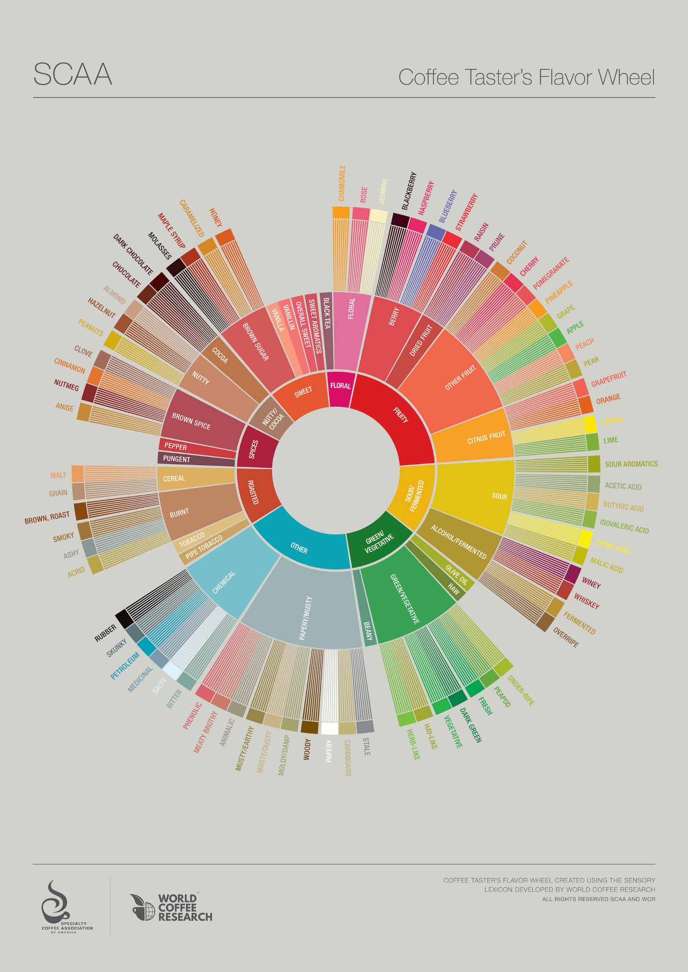
Consider our final example of a Sunburst chart. Figure 12 above depicts a coffee tasters flavour wheel. In terms of colour, a wealth of shades are used. The inner segment contains nine distinct colours, the middle segment contains twenty-eight colours, while the outer segment contains over seventy colours. You may recall from our Sankey chart discussion the use of many colours may introduce readability concerns.
Due to the layout of the colour scheme and category placement, the red, orange and yellow hues are placed in the upper half of the wheel, while the blue, green and grey hues are positions in the lower half of the wheel. There is some ‘colour crossing’ on the outer segment of the wheel, most notably some brown and green hues, however as the chart is meant to be read from the centre outwards, the juxtaposition of colour is less noticeable.
Sunburst charts are a very popular type of chart, that allows for a level of interaction. Implements are available across a wide range of frameworks. In addition to the frameworks previously mentioned, Sunburst charts can be created in Microsoft Office and SPSS.
Conclusion
In summary, four types of charts for displaying flows between categorical data were discussed. Each chart type has its own unique quality for visual storytelling.
An Arc Diagram is useful at mapping 1:1 entity-relationships. Applications of such a chart include plotting the relationships of notes used in Beethoven’s Für Elise, to the character interactions in Les Misérables.
A chord diagram is used to display the strength of inter-relationships between categories. The thicker the chord, the stronger the relationship. One application of a chord diagram considers the relation between the count of words spoken between characters in the TV show Friends.
Sankey charts were shown to plot the multi-flow relationships between categories and can also be used to show the process flows between multi-component systems (e.g a steam engine)
Finally, a sunburst chart is used to plot event sequences and their proportional relationships as part of a wider set of relationships. Whether understanding the page-sequence flows on a website or the sequence of coffee flavours, a sunburst chart can cover it.
For all their differences, each chart types provides a unique way to tell a visual story with categorical data and their associated counts. Let the charts flow.
I work as a Data Scientist by day, and have a passion for visual story telling. I have a PhD in Mathematics and Statistics and love watching Cricket.
- Jonathan Dunne


