
Two ways a single number hides how a climate dataset actually behaves, and what I did about each
I built a map that ranked cities by one number: how many daylight hours in a typical year are comfortable for being outside. It looked right. It was also, in a way that took me too long to notice, the wrong picture.
The dataset covers 478 cities. For every city and month, it counts the daylight hours when it is neither too hot, too cold, too wet, nor too windy to be outdoors, and it attributes every lost hour to one of those four causes (Wackher 2026, doi:10.5281/zenodo.21976372). That structure gave me two design problems, one continuous and one categorical. Neither was solved by the obvious chart.
Problem one: The total hides the year
Take Berlin, Phoenix, and Bandung, in Indonesia. Their yearly totals are 2,353, 2,372, and 2,332 hours. The biggest gap between any two of them is 40 hours, which is 1.7% of the smallest total. Rank them by the annual number and they’re a tie.
They are not remotely the same place to live. Figure 2 shows the monthly profiles. Berlin has no comfortable hours in January, February, or December, and 451 in July. Phoenix is the mirror image: 331 hours in April, then 38 in July and 36 in August, when the heat takes the daylight. Bandung hardly moves at all, from 162 hours in its worst month to 235 in its best.

Bogotá is the flat extreme. Its months run from 282 to 317, a swing of 35 hours across the whole year, while Berlin’s swing is 451.
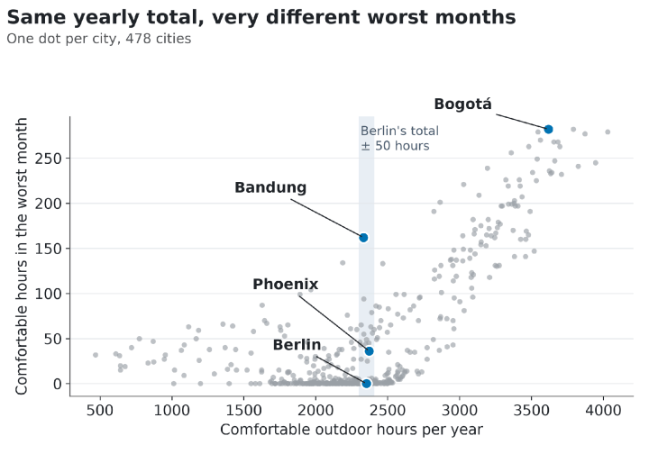
Is this just three handpicked cities? Figure 1 says no. I plotted each city’s yearly total against its worst month. Across all 478, the two are correlated (r = 0.72), so the total isn’t useless. But look at the shaded band around Berlin’s total. It holds 56 cities. In 49 of them, the worst month has fewer than 50 comfortable hours. Only one has a worst month of 150 or more, and that one is Bandung. Pick any total in the middle of the range and you are choosing among very different calendars.
At the dataset level, 333 of the 478 cities have at least one month under 50 comfortable hours, and 130 have a month at zero. A single yearly figure, mapped, says nothing about this.
What I tried first
I’ll be straightforward about the first two maps most people would build, because I built them again for this article to see how bad they are. Figure 3 shows both.

The top map is the single-number version. The mid-range greys all look alike, which is exactly where the cities with very different calendars live. A sequential scale can only tell you where something is high or low. It can’t tell you what shape the year has.
Small multiples, as in Figure 2, are the right fix for any one city, but they don’t scale to a map of 478. A seasonal summary on the map, such as the swing between best and worst month, would help. But it throws away which months, and a city that’s good in July and one that’s good in January stop being distinguishable. So I stopped asking the map to carry the shape of the year. The map finds a place. The monthly profile, one click away, describes it. Those are two jobs, and a single chart does neither well.
Problem two: four causes, wildly unequal
The second problem arrived when I started to attribute lost hours. For each city, I could now say how many daylight hours were lost to heat, cold, rain, and wind, and the interesting question became which one binds. I coloured each city by its largest loss (the bottom map in Figure 3).
Counted that way, cold binds in 310 of 478 cities, heat in 156, rain in six, and wind in six. One city, Tulsa, has an exact tie between heat and cold, and my count assigns it to heat. So cold is about 65% of the map, heat about 33%, and rain and wind together 2.5%.
That is an encoding headache. Four categories are easy to colour, but at those frequencies, the last two are specks. Making them bigger distorts the map. Adding labels to specks doesn’t fix the underlying problem, which is that the legend implies four comparable categories when the data holds two common ones and two rare ones. And “binds” overstates the case in many places. In 79 cities, or 17%, the runner-up cause costs at least half as much as the leader. A solid colour hides that.
Treat the wind count with care. The wind term is the least trustworthy in the dataset (more on that below), so the six wind-binding cities are the category I trust least. I won’t name them or build anything on them.
What I ended up with
Figure 4 plots hours lost to cold against hours lost to heat for every city except the six where wind binds, with the diagonal marking a tie. The colour still says which cause binds, but now you can see the structure the map hid. The data forms an L. Cities mostly hug the vertical axis (heat but little cold) or the horizontal axis (cold but little heat), with losses as high as 3,722 hours to heat and 3,281 to cold. Ninety cities lose at least 300 hours to both, which is why the middle of the plot isn’t empty.

The rain cities now explain themselves. They sit near the origin because they lose few hours to heat or cold. The median city where heat binds loses 1,636 hours to heat; where cold binds, 1,773 to cold. Where rain binds, the median loss to rain is 484. Rain binds because the other causes are small, not because the rain is severe. Medellín, for example, loses 618 hours to rain, 236 to heat, and 28 to cold, and still finishes the year with 3,545 comfortable hours.
Rather than force four categories into one map, I now treat the two common causes as the main axes and show rain as what it is: a minor constraint that decides a handful of places. Wind I leave out of any per-city display, for the reason below.
What I’d tell you to take from this
If your dataset has a time dimension, then the annual total is a summary you earn the right to show, not the default. Check whether similar totals hide different shapes before you rank anything by it. If your dataset has a categorical breakdown with very uneven frequencies, don’t make the map carry it. Show the continuous quantities underneath, where small categories fall out of the geometry rather than fighting for pixels.
Limitations
The comfort band is my judgement, not a standard. I count a daylight hour as comfortable when apparent temperature sits between 10°C and 29°C, applied probabilistically rather than as a hard cutoff. Move the band and every absolute number moves. The ordering of cities moves much less, because the same rule applies everywhere, but I haven’t proved that here.
The wind term is calibrated in aggregate against 624 weather stations, and it is not resolved at city scale. It is right on average, not city by city. That’s why I keep the wind-binding category out of every conclusion and every per-city chart above, and why you shouldn’t read a single city’s wind loss as a measurement.
Finally, these are 1981–2010 climatological averages, not forecasts, and a “typical year” never actually occurs.
Data and methods
Every figure in this article comes from the per-city table of the dataset: comfortable daylight hours for each month, and hours lost per year to heat, cold, rain, and wind. The dataset is open under CC BY 4.0 and archived with a DOI, so the numbers here can be checked against a fixed version (Wackher 2026, doi:10.5281/zenodo.21976372). If you want the raw per-city table rather than the archive, it’s served at georank.place as JSON.
The charts were made in Python with Matplotlib, using the colour-blind-safe Okabe-Ito palette. The script that produces every chart and number is available on request.

Christoph Wackher
Christoph Wackher maintains the GeoRank dataset andgeorank.placeindependently, building tools for comparing places to live and writing about the data behind them.


